LectroTIC-4 — 4-Channel Pulse Timestamper

A four-channel zero-dead-time pulse timestamper with 4-nanosecond resolution. Plug it into your USB port, feed it pulses, and it streams a list of the times each pulse arrived, accurate to a few nanoseconds against your lab's reference clock.

The 4-channel timestamper.

Overview

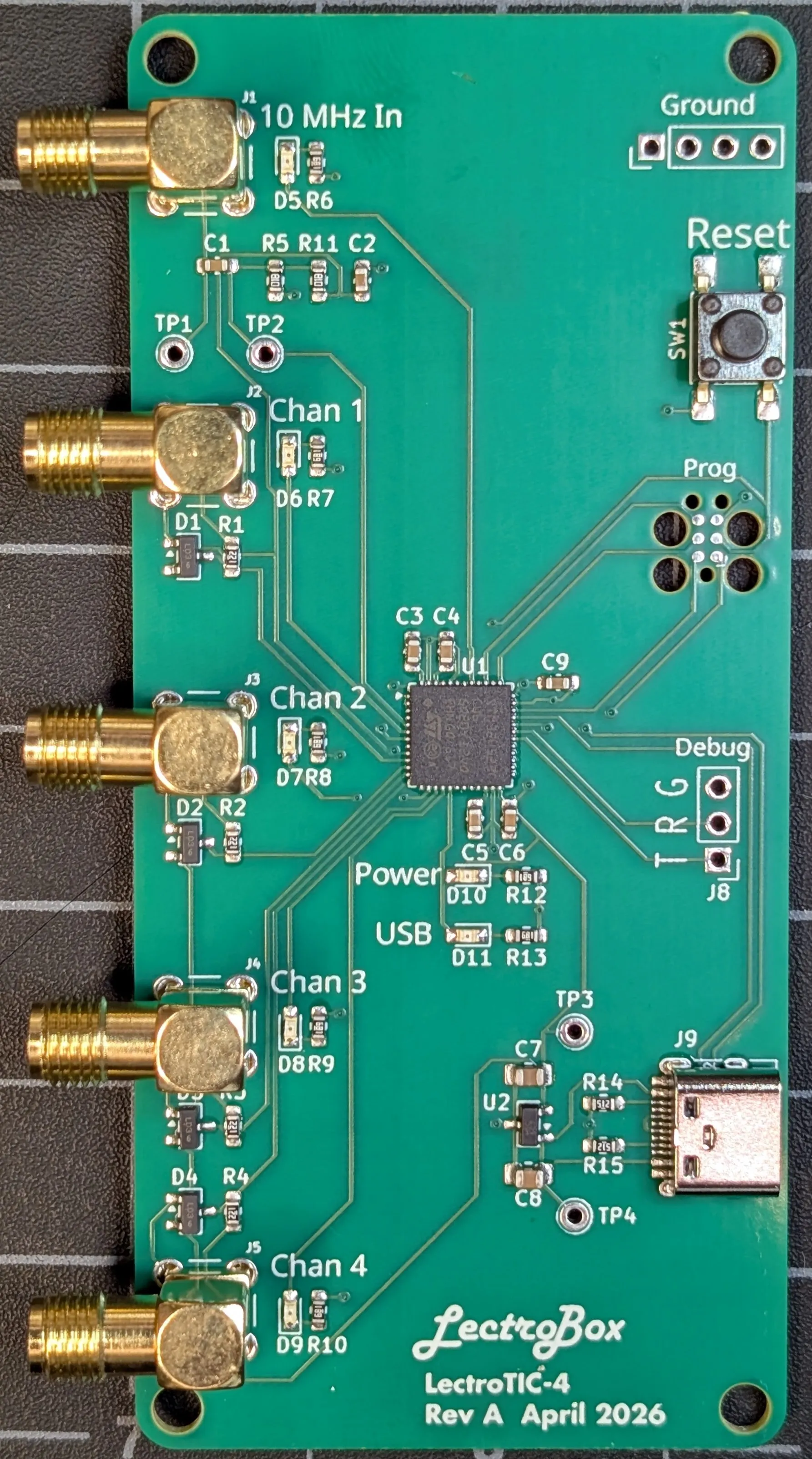
The LectroTIC-4 records the precise moment a pulse arrives on any of its four inputs and sends a stream of timestamps out over USB. Resolution is 4 nanoseconds, and the absolute accuracy is whatever your reference oscillator is — a rubidium standard, a GPS-disciplined oscillator, or any other 10 MHz source you trust.

It is zero-dead-time: the timescale never stops, restarts, or loses precision while the device is running. Every pulse you capture sits on the same continuous nanosecond-resolution timeline (the timeline starts at zero at power-up and counts forward indefinitely), whether the pulse arrived a microsecond or a year after the previous one.

The four channels are also coherent: they all sample against the same clock and the same counter, so a timestamp on CH 1 and a timestamp on CH 3 can be subtracted directly to get the true time difference between the two pulses — there is no per-channel clock or counter that could drift. That makes the device suitable for long unattended runs where you need to know not just when each pulse occurred but also how each pulse relates to every other pulse seen across all four channels.

Each channel can be independently configured for rising-edge, falling-edge, or both-edge capture (use both edges to time a pulse’s width directly) and for an optional integer divider that reports only every Nth pulse — useful for downsampling busy inputs or matching a reference channel’s rate. These settings are available through a small SCPI command set on the same USB connection.

It is also high throughput. The on-device buffer captures pulses as little as 4 ns apart on a single channel for the first 4,096 pulses, and as little as 150 ns apart for the next 12,288 (16,384 timestamps total before the host must drain the buffer) — orders of magnitude faster than the burst rates most laboratory time-interval counters can sustain. Once the buffer is in steady state the host becomes the bottleneck: the default ASCII output streams at roughly 25,000 timestamps per second, and an optional compact binary mode (selectable with a single SCPI command) pushes that to about 100,000 per second, near the practical ceiling of a USB Full-Speed link.

It is also designed to be easy to use: the device connects over USB and enumerates as a standard virtual serial port on Linux, macOS, and Windows. There is nothing to install on the host — no driver, no companion app, no SDK — and the device emits plain ASCII text, one timestamp per line, that you can read with any terminal program or pipe directly into a script. The defaults (rising edge, divider 1, all four channels active) are sensible enough that no configuration is required for first-time use; the SCPI commands are there if and when you want them.

Basic usage

1. Connect a 10 MHz reference clock (rubidium, GPS-disciplined, or any other stable source) to the 10 MHz In input.
2. Plug the device into a USB port on your computer. The 10 MHz indicator LED begins flashing once the reference clock is locked. The reference clock is checked once at boot, so if you change or reconnect the source after the device is already powered, press the RESET button to make it re-lock — no need to unplug USB.
3. Open the virtual serial port the device created — /dev/ttyACM* on Linux, /dev/cu.usbmodem* on macOS, or a new COM port on Windows.
4. Connect signals to any of the four SMA inputs (CH 1 … CH 4) and timestamps will stream to your terminal program over USB.

Pulse requirements

By default each channel timestamps the rising edge of each pulse — the moment the input goes from LOW to HIGH. The polarity is selectable per channel via the SCPI command INPut<n>:SLOPe POSitive|NEGative|BOTH (see Command interface below). Falling-edge mode captures HIGH→LOW transitions instead; both-edge mode captures both, which lets you measure pulse widths directly by subtracting consecutive timestamps on the same channel. The minimum reliable pulse width is 4 ns in any mode; anything narrower may be missed. Slow edges are tolerated thanks to the input’s ~250 mV of Schmitt-trigger hysteresis, but extremely slow ramps (below a few mV/ns) may produce duplicate triggers as the signal crosses the threshold band.

The input registers as low for voltages below ~1.0 V and as high for voltages above ~2.3 V, so a standard 3.3 V or 5 V CMOS-level pulse train works directly. Each input is protected by a 220 Ω series resistor and a BAT54S clamp to the 3.3 V rail and ground, which absorbs continuous inputs up to 12 V and brief overshoots well beyond that without damage.

Output format

The device sends a stream of plain ASCII text terminated by a single \n (LF) per line. No carriage returns, no binary framing, no driver. Output looks like this:

# Starting timestamper, version 9afaa32f
1 5293.585203496
1 5293.587201024
3 5293.601004112
1 5293.589198608
2 5293.601100008

Each timestamp line is <channel> <seconds>.<nanoseconds>. The seconds counter starts at zero when the device powers up and counts forward indefinitely (it doesn’t wrap until ~136 years). Channel numbers are 1 through 4.

Any line that starts with # is a status message rather than a timestamp:

• # Starting timestamper, version <git-hash> — printed once after USB enumeration and the reference clock locks. The git hash identifies which firmware build is running.
• # FATAL: External oscillator failure. Connect a 10MHz source and press reset. — printed once if the reference clock fails to start at boot, or drops out mid-run. The device stops emitting timestamps until reset.
• # ch<N>: <X> overcaptures, <Y> buf overflows — printed when a channel’s pulse rate exceeded what the device could handle. The two counters are distinct failure modes. Overcaptures count pulses that arrived closer together than the minimum event interval, so a new capture stomped on the previous one before it could be recorded. Buf overflows count pulses dropped because the 16,384-timestamp internal buffer filled faster than USB could drain it. To eliminate overcaptures, space your pulses further apart; to eliminate buf overflows, reduce the average rate or split your work into bursts of ≤ 16,384 pulses with quiet periods between to let the buffer drain.

If the reference clock fails

The reference clock is checked once at boot and continuously monitored afterward. If the 10 MHz signal disappears or drifts out of range:

1. The 10 MHz LED goes dark.
2. The device emits the # FATAL line above on USB.
3. Timestamping halts. No further timestamps appear, even if pulses are arriving on the inputs — the device refuses to operate without a trusted reference, since any timestamps it produced would be wrong.

To recover, restore the 10 MHz signal at the 10 MHz In input and press RESET. There’s no need to unplug USB.

Indicator LEDs

10 MHz

• Dark: reference clock missing or failed. The device will refuse to emit timestamps until you restore the reference and reset.
• Continuous blink: reference clock locked, device is timing.

USB

• Dark: nothing on the host has opened the device’s serial port — this is the state both when the cable is unplugged and when it’s plugged in but no program is reading
• Solid: a host program has opened the port
• Blinking: data is flowing to that host program

CH 1–CH 4 (one per channel)

• Dark: no pulses arriving
• Periodic blink: a pulse has arrived
• Continuous blink: pulses are arriving at >5 Hz

Command interface

The timestamper accepts SCPI-style commands on the same USB CDC port it streams timestamps over. Sending commands is strictly optional: out of the box, the device starts streaming on plug-in with all four channels in rising-edge capture mode and no divider, and you never need to send anything to use it. Commands are only there for users who want to change those defaults — invert a channel’s edge polarity, set a divider, suppress streaming during a synchronous query session, or switch the output stream to a compact binary format that roughly quadruples the sustainable record rate (see FORMat:DATA below).

Send a single command line (terminated with \n); the device responds with silence for setters, one line of data for queries, or latches an error that you can read back later. Commands are case-insensitive and accept either the standard SCPI long form or the abbreviated short form (the capital letters in each keyword name).

Standard IEEE 488.2 commands:

Per-channel input configuration (channel suffix <n> is 1, 2, 3, or 4; if you omit it the command operates on channel 1):

Streaming output:

Example session:

*IDN?
Lectrobox,Timestamper,0,9afaa32f

INP2:SLOP NEG
INP3:DIV 100

INP2:SLOP?
NEG
INP3:DIV?
100

*RST
INP2:SLOP?
POS
INP3:DIV?
1

Commands and timestamp data share the stream, so if you send a query while pulses are flowing, the response line will appear inline with the timestamps. To get a clean back-and-forth, send OUTPut:STATe OFF first to pause the timestamp stream, run your queries, then OUTPut:STATe ON to resume; the device buffers up to 16,384 timestamps internally during the pause and drains them when streaming resumes.

Terminal programs

Any program that can read a serial port works. All of the suggestions below are free and open-source.

• Linux
  • grabserial (pip install grabserial) — Python command-line tool that logs serial output with a host-side timestamp on each line; great for capture-to-file. Run as grabserial -d /dev/ttyACM0.
  • pyserial-miniterm /dev/ttyACM0 (comes with the pyserial package).
  • picocom — a small, friendly terminal: picocom /dev/ttyACM0.
  • minicom — older but common and capable.
  • screen /dev/ttyACM0 — built into most distros.
  • cat /dev/ttyACM0 — see the line-discipline note below first.

  Linux opens new serial ports in canonical mode, which echoes incoming characters back out to the device — fine for an interactive shell, but it can corrupt the timestamp stream. Programs designed for serial work (grabserial, pyserial-miniterm, picocom, minicom, screen, and our own tsctl.py) reconfigure the port automatically and need no setup. Simpler tools like cat do not, so before using them, run:

  stty -F /dev/ttyACM0 raw -echo
  

  To make this permanent, drop the following into /etc/udev/rules.d/60-lectrotic.rules and run sudo udevadm control --reload:

  SUBSYSTEM=="tty", ATTRS{idVendor}=="1209", ATTRS{idProduct}=="71c4", \
      RUN+="/usr/bin/stty -F /dev/%k raw -echo", \
      SYMLINK+="lectrotic-4"
  

  The SYMLINK line also gives you a stable /dev/lectrotic-4 device node so you don’t have to guess whether your timestamper came up as /dev/ttyACM0 or /dev/ttyACM1.

• macOS
  • grabserial and pyserial-miniterm install the same way as on Linux (via pip).
  • picocom and minicom are available via Homebrew: brew install picocom minicom.
  • screen /dev/cu.usbmodem* — built in.
  • cat /dev/cu.usbmodem* — see the line-discipline note below first.

  macOS has the same default line-discipline behavior as Linux, so before using cat you’ll want to run stty -f /dev/cu.usbmodem* raw -echo (note -f instead of Linux’s -F). The dedicated serial programs above handle this automatically.

• Windows
  • PuTTY — pick “Serial,” type the COM port name (e.g. COM5), click Open.
  • Tera Term — open-source terminal with a clean serial-port dialog.
  • pyserial-miniterm COM5 and grabserial -d COM5 work the same as on Linux/macOS once you have Python installed.

tsctl: a one-file Python utility

Any of the terminal programs above are fine for casual use, but if you want a more convenient way to send SCPI commands and get the higher throughput that binary mode unlocks, tsctl.py is a small, self-contained Python script (the only dependency is pyserial) that wraps the SCPI interface and the streaming output behind a friendly command line. Save the file, chmod +x, and run.

It auto-detects the LectroTIC-4 by USB VID/PID (no --port needed unless you want to override), and provides subcommands for everything the device exposes:

• tsctl.py idn — read *IDN?
• tsctl.py reset — *RST
• tsctl.py slope <ch> [POS|NEG|BOTH] — set or query slope
• tsctl.py div <ch> [N] — set or query the divider
• tsctl.py output [ON|OFF] — set or query streaming
• tsctl.py raw '<scpi>' — send any SCPI command verbatim
• tsctl.py stream — forward the timestamp stream to stdout

The stream subcommand is the most useful one for everyday use. By default it puts the device into binary output mode (the high-throughput 8-byte-per-timestamp wire format described above), then decodes those records back into the same human-readable <channel> <seconds>.<nanoseconds> ASCII lines you’d see in the default text mode — so you get the throughput benefit of binary without changing what your downstream pipeline reads. Pass tsctl.py stream text to forward the raw text stream instead, and on exit it always restores the device to text mode for any other tool that comes along next.

Two extra niceties: tsctl.py configures the serial port for raw / no-echo operation itself (no stty needed), and on Linux it works regardless of which /dev/ttyACM* the kernel happened to assign.

tsctl.py is also a small Python library — drop it next to your own script (or pip install directly from the URL), from tsctl import Timestamper, and you have an autodetecting, context-managed handle to the device with method-style access to every SCPI feature plus the high-throughput binary stream:

from tsctl import Timestamper

with Timestamper() as ts:                    # autodetect
    print(ts.idn())
    ts.reset()
    ts.set_slope(1, "BOTH")
    ts.set_divider(1, 100)                   # one stamp per 100 edges
    ts.set_format(binary=True)
    ts.set_stream_enabled(True)
    for r in ts.read_for(5.0, binary=True):
        if r.kind == "ts":
            print(f"channel {r.channel}: {r.time:.9f} s")

read_for(duration, binary) is a generator that yields Record named tuples with fields (kind, channel, time, comment). For an edge capture, kind == "ts", channel is 1–4, time is a float giving seconds since the device booted, and comment is None. In text mode the device also emits diagnostic lines (overflow / boot banner / etc.) which arrive as records with kind == "comment" and the line text in comment. Binary mode suppresses comments. The generator exits cleanly after the given wall-clock window, even if the device is silent, so you can wrap timestamp capture in your own measurement logic without touching pyserial directly. The regression test, deadtime sweep, and sustained-rate sweep under src/app/timestamper/util/ are larger worked examples of the same library.

Comparison to similar instruments

Most time-interval counters — from the legendary HP 5370A/B (1979, 20 ps single-shot, still the gold standard in the time-nuts community) through the modern Pendulum CNT-91 — use analog interpolation: charging a capacitor between the input edge and the next clock tick, digitising the resulting voltage, and reconstructing the sub-clock fraction of the time interval. The HP and Pendulum instruments call this a “vernier interpolator,” the SR620 calls it a time-amplitude converter, the Keysight 53230A calls it a multi-stage time interpolator, and the TAPR TICC delegates to a TI TDC7200 chip that does the same job in silicon. This technique gets ps-class single-shot resolution, but the analog stage takes finite time to charge, digitise, and reset — so those instruments trade sample rate against resolution. The higher the single-shot resolution, the lower the back-to-back capture rate the analog stage can sustain.

We chose the opposite trade-off. The timestamper has no analog interpolator at all — it just runs a 32-bit hardware counter at 250 MHz and snapshots it on every input edge via DMA. That floors single-shot resolution at one clock tick (4 ns) but lets the device record edges as fast as they arrive, in bursts at the timer’s full hardware rate, with no per-sample dead time. If you need ps-class resolution on a single edge, one of the instruments in the table below is the right tool. If you need to capture every edge of a high-rate train, four channels at once, on a continuous coherent timeline, this is the right tool.

Two instruments above are open-source: the TAPR TICC (designed for the amateur time-and-frequency community by John Ackermann N8UR), and this timestamper. Everything else is a closed proprietary instrument. Of the proprietary instruments, the HP 5370A/B, 5335A, and 5371A/5372A are out of production but readily available on the secondary market; the SR620, 53230A, CNT-91, and CNT-104S are still in current production from their respective manufacturers.

The Pendulum CNT-104S is the only other instrument in the table with four input channels and gap-free time-stamping on all of them — and Pendulum explicitly markets it for the same use case (phase comparison of four atomic clocks) at roughly 140× the price of the LectroTIC-4. The HP 5371A/5372A are the vintage instruments most likely to come up when time-and-frequency hobbyists want fast, continuous capture at modest single-shot precision; their 10–13 MSa/s continuous mode is the closest entry in the table to the LectroTIC-4’s burst rate, but only on a single channel and only in a measurement session bounded by the instrument’s capture memory.

In short: the eight instruments above are precision laboratory tools for measuring an individual event with picosecond-class accuracy. The timestamper is a streaming recorder for measuring every event in a continuous train across four coherent channels, at the resolution ceiling of what an STM32H523’s hardware counter can offer in pure digital silicon.

Specifications

Channels and timing

Inputs

Reference clock and host interface

Physical and environmental

Schematics, Software, and Other Sundries

The hardware design and firmware are open-source.

• Firmware: src/app/timestamper/ in the RULOS project on GitHub.
• Schematics, BOM, and PCB layout: coming soon.

Join the Conversation